Spring 2023 test solutions overview

20 minute read

Published: May 16, 2023

In this post we will go through the questions that were a part of the Spring 2023 written test, one of the steps of the MALTO selection process. We will go through the texts and we will present a solution.

Let’s start with the simple questions, which could be easily addressed with a basic knowledge of machine learning algorithms.

Question 1

Text A decision tree is a machine learning algorithm that builds a decision graph, in which each node performs a decision based on a feature’s value (e.g., considering the iris dataset, a dataset about flowers, a node may split data considering “petal length > X”). The training process evaluates different splits by computing an impurity measures on training data, generating the aforementioned nodes and the resulting model. Usually, a limit on the depth of the tree structure can be defined. What happens if no such limit is enforced, i.e., the decision trees grows to its maximum depth?

The resulting model is more complex but achieves similar performances
Better performances are achieved. Such constraints are present in order to avoid long training time
No conclusions can be drawn without any information about the dataset
The resulting model will typically overfit the training data
The algorithm cannot converge and will be stuck in an infinite loop
None of the other answers is correct

Solution Now, a decision tree that fits the entire dataset will grow to make some decisions (splits) based on very few points. Learning a dataset to such extremes is bound to bring overfitting problems, so the correct answer is 4 (The resulting model will typically overfit the training data).

Question 2

Text You have a machine learning algorithm which is performing very well on train data, but extremely poorly on test data. What could be the most probable cause?

The algorithm may be overfitting on the training data
The algorithm may be underfitting the training data
None of the other answers is correct
The chosen machine learning algorithm should be changed to a more performing one
A wrong configuration of the machine learning algorithm

Solution Another very simple question about the basics of machine learning. It is a well-known fact that models may overfit the training data: this occurs when a model learns a bit too well the training set (thus performing well on it), but fails to generalize to new (e.g. test) data. Therefore the answer is 1 (The algorithm may be overfitting on the training data).

Question 3

Text You are given an array containing integer numbers and an integer value N. You want to write a program to determine whether or not exactly the sum of two distinct elements contained in the array is equal to N. Such program must return either True or False. Which is the lowest possible complexity you can achieve?

Example: [1, 4, 5, 4, 8, 9, 25], N = 8. Answer: True, because 4 (index 1) + 4 (index 3) = 8.

O(1)
O(log(n))
O(n)
O(n*log(n))
O(n^2)
None of the other answers is correct

Solution The simplest solution to this problem is O(n^2): we iterate over every possible pair of values in the list and check their sum. But we can probably do better than this.

Another O(n^2) solution is the following:

l = [1, 4, 5, 4, 8, 9, 25]
N = 8
for el in l:
    if l.count(N-el) > int(N-el == el):
        print("Found", el, N-el)

Note the following:

The if condition makes sure that we also handle situations where two identical numbers produce N when summed. The provided example works because “4” appears twice. The problem [1, 4, 5, 8, 9, 25] would not work because “4” only appears once. Hence we check that the count of N-el is > 0 if we are searching for two different numbers, otherwise we check that the count is > 1 [ note: int(False) = 0, int(True) = 1 – additionally, the int() casting was not necessary and only used to make the code more intuitive].
The O(n^2) comes from the l.count() operation, which goes through the list to count the number of occurrences.

However, we could pre-compute the counts of all elements once before the checks (going through the list once, O(n)). If we store the counts inside of a dictionary (O(1) search cost), we can build a solution in O(n).

l = [1, 4, 5, 4, 8, 9, 25]
N = 8
counts = defaultdict(lambda: 0, Counter(l)) # O(n)
for el in l: # O(n)
    if counts[N-el] > int(N-el == el): # O(1)
        print("Found", el, N-el)

(Note: Counter and defaultdict come from the collections module and are used for convenience, with a few additional lines the same result could be achieved).

Long story short, the solution can be O(n) (answer 3).

Question 4

Text

recall(X) is the fraction of correct predictions among the samples with actual class X
precision(X) is the fraction of correct predictions among the samples predicted with class X

A random forest classifier has been trained on a 2-dimensional dataset (features x1, x2). Each point in the dataset is labelled as either A, B or C (star, cross, triangle respectively).

The following figure represents a test set that is used to validate the classifier.

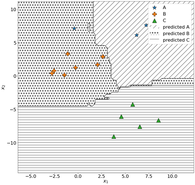
The decision boundaries of the model are shown in the figure:

Diagonal lines represent areas of the input space where the model predicts class A
Small circles represent areas of the input space where the model predicts class B
Horizontal lines represent areas of the input space where the model predicts class C

Write in the box below precision(B) and recall(A), separated by a comma.

For example, if precision(B) = 0.2 and recall(A) = 0.5, write 0.2,0.5 (order matters!). Use at least 4 significant figures.

Solution This exercise is a matter of understanding the definitions of precision and recall (provided as a part of the exercise) and interpreting the provided image.

We can easily see that we predict a total of 8 points as “B”: 7 are actually of class B (orange crosses), whereas one is a blue star (A). Therefore, the precision for B is 7/8 = 0.875.

As for A, we notice that we correctly predicted 2 points, whereas we were supposed to predict 3 of them (one was mispredicted as B). This implies a recall of 2/3 = 0.6667.

Question 5

Text A 1-dimensional dataset is used for learning the weights of a linear regression model. The data used and the model obtained are shown in the figure below (top-most figure – “Data/model plot”).

We define the residual ri for the i-th point (xi, yi), with prediction y’i, as ri = yi - y’i.

Based on this definition, which of the following plots correctly represents the residuals for the top-most figure (x values on the x axis, residuals on the y axis)?

Note: The x and y labels and values have been removed on purpose. The x axis contains the values of the 1-dimensional features of the dataset (independent variable), whereas the y axis represents the target variable y (dependent variable).

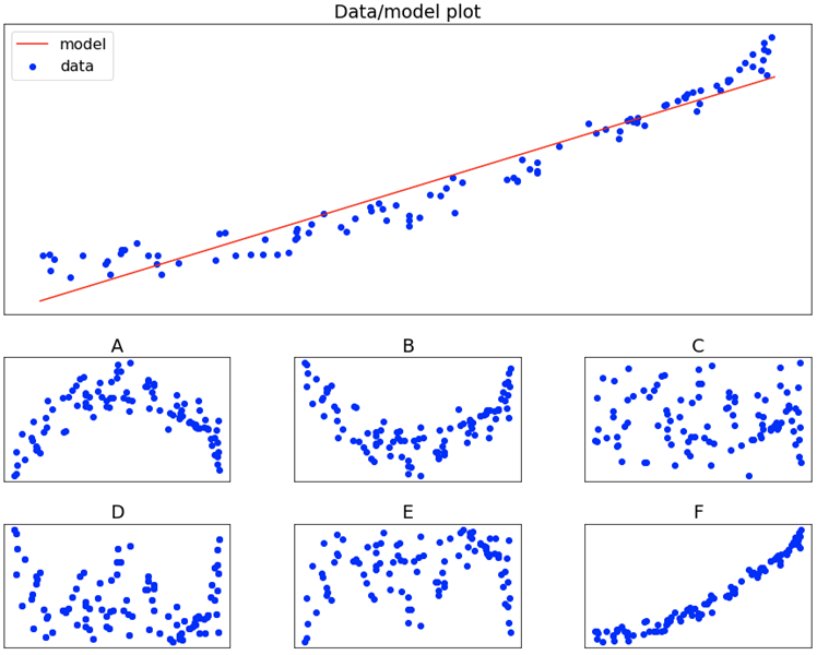
Solution We can easily solve this exercise by looking at the tails of the the data/model plot, as well as its center. We notice, along the tails, that the actual values (y_i) are larger than the predictions (the model is underestimating the targets). This implies that the residuals (as defined in the text of the exercise) will be positive. Similarly, for central values, the model is overestimating the target (the targets are below the model predictions). This implies that residuals will be negative.

The only plot that clearly reflects this trend (tails greater than the middle) is the one depicted in figure B. All others are in one way or another incorrect.

Question 6

Text You are given the following PyTorch CNN-based model.

You want to feed a batch of size 512, each representing a black/white image of 256x256 pixels – in other words, the batch shape is (512, 1, 256, 256).

What is the correct value for the parameter M to be passed to the constructor?

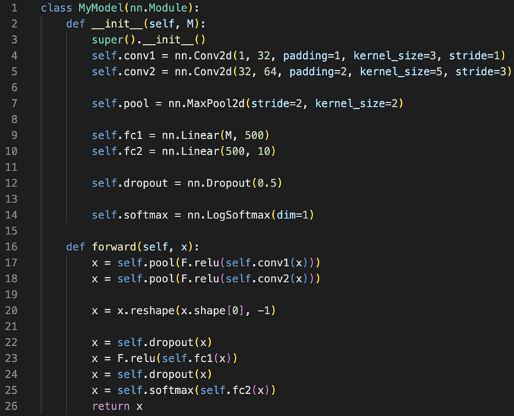
Solution One possible solution for this exercise was to manually compute the size of the feature maps obtained after each convolution. This is a rather time-consuming and error-prone way of proceeding – let’s be honest: almost nobody would go that way!

We could instead copy the first portion of the model (yes – it was a screenshot to make your life a bit harder :D) and extract (“print”) the shape of x where we are interested.

class MyModel(nn.Module):
    def __init__(self):
        super().__init__()
        self.conv1 = nn.Conv2d(1,32, padding=1, kernel_size=3, stride=1)
        self.conv2 = nn.Conv2d(32,64, padding=1, kernel_size=3, stride=1)
        self.pool = nn.MaxPool2d(2,2)

    def forward(self, x):
        x = self.pool(F.relu(self.conv1(x)))
        x = self.pool(F.relu(self.conv2(x)))
        x = x.reshape(x.shape[0], -1)
        print(x.shape)
        return x

We can then create the model and call it with a batch having the right shape (note that the batch size did non affect the answer!):

x = torch.rand((512, 1, 256, 256))
model = MyModel()
model(x)

Which returns torch.Size([512, 262144]), hence 262144 was the correct answer! (512 being the batch size).

Question 7

Text For a binary classification problem, you are given the ground truths for a batch of 16 points. You additionally receive the predictions for those 16 points, in terms of probability for the positive class p(1|x).

y_true = [0, 0, 1, 1, 0, 1, 0, 0, 1, 0, 1, 1, 1, 1, 0, 1] y_pred = [0.2628, 0.8054, 0.5164, 0.3188, 0.7841, 0.0636, 0.3322, 0.2479, 0.0226, 0.0260, 0.7305, 0.6972, 0.0105, 0.8633, 0.5260, 0.5806]

For a point x with ground truth y and predicted value y’, the binary cross entropy BCE(y, y’) is defined by the formula below.

$BCE(y, y’) = -y log (y’) - (1 - y) log(1 - y’)$

What is the mean binary cross entropy over the batch?

None of the other answers is correct
0.9470
0.7848
1.1938
1.2004
0.8741

Solution This exercise can be easily solved using NumPy arrays, by applying the BCE formula to each sample and then averaging over the batch:

y_true = np.array([0, 0, 1, 1, 0, 1, 0, 0, 1, 0, 1, 1, 1, 1, 0, 1])
y_pred  = np.array([0.2628, 0.8054, 0.5164, 0.3188, 0.7841, 0.0636, 0.3322, 0.2479,  0.0226, 0.0260, 0.7305, 0.6972, 0.0105, 0.8633, 0.5260, 0.5806])
print(-(y_true * np.log(y_pred) + (1 - y_true) * np.log(1 - y_pred)).mean())

Alternatively, we could have used PyTorch’s already implemented BCE loss function:

y_true = torch.tensor([0, 0, 1, 1, 0, 1, 0, 0, 1, 0, 1, 1, 1, 1, 0, 1]).float()
y_pred  = torch.tensor([0.2628, 0.8054, 0.5164, 0.3188, 0.7841, 0.0636, 0.3322, 0.2479,  0.0226, 0.0260, 0.7305, 0.6972, 0.0105, 0.8633, 0.5260, 0.5806])
print(nn.BCELoss()(y_pred, y_true))

Question 8

Text Given the binary classification dataset contained in the link below, try several different classifier in order to achieve the best possible accuracy score without any preprocessing operation.

https://gist.githubusercontent.com/lccol/3ab34ae5b93aff96dc4ae68e73e6d12b/raw/8b02713ee2364914eb17cd0de4b0eebb0fd4a797/question_dataset.csv

Note: you can easily read the csv given the link directly from pandas import pandas as pd url = “https://…” df = pd.read_csv(url)

Is there any classifier which achieves best overall performances compared to the others?

SVM classifier with sigmoid kernel and C=0.001
SVM classifier with linear kernel and C = 1.0
Logistic Regression with L1 penalty and balanced class weights
Logistic Regression with L2 penalty and {0: 0.5, 1: 10} class weights
None of the specified classifiers has a clear advantage with respect to the others
SVM classifier with rbf kernel and C = 1.0

Solution We can approach this problem in two ways. We can either visualize the data and infer the most suitable classifier, or we can try all classifiers.

For the first option, two lines of code were sufficient:

df = pd.read_csv("https://gist.githubusercontent.com/lccol/3ab34ae5b93aff96dc4ae68e73e6d12b/raw/8b02713ee2364914eb17cd0de4b0eebb0fd4a797/question_dataset.csv")
plt.scatter(df.x, df.y, c=df.label)

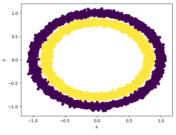
From this, it easily follows that the only suitable classifier among the ones proposed is an SVM that makes use of an RBF kernel.

Alternatively, we could have measured the accuracy of all proposed classifiers (of course, on a test split):

X_train, X_test, y_train, y_test = train_test_split(df[["x","y"]], df["label"], train_size=.8)
models = [
    SVC(C=0.001, kernel="sigmoid"),
    SVC(C=1.0, kernel="linear"),
    LogisticRegression(penalty="l1", class_weight="balanced", solver="liblinear"), # liblinear needed for to use an l1 penalty
    LogisticRegression(penalty="l2", class_weight={0: 0.5, 1: 10}),
    SVC(C=1.0, kernel="rbf")
]

for model in models:
    model.fit(X_train, y_train)
    print(model, accuracy_score(y_test, model.predict(X_test)))

From that, we obtain the following results:

SVC(C=0.001, kernel='sigmoid') 0.4915
SVC(kernel='linear') 0.4915
LogisticRegression(class_weight='balanced', penalty='l1', solver='liblinear') 0.507
LogisticRegression(class_weight={0: 0.5, 1: 10}) 0.4915
SVC() 0.9995

Making it clear that the SVM with RBF kernel is the only model that performs better than chance (and actually solves the problem almost perfectly) – making 6 the right answer (SVM classifier with rbf kernel and C = 1.0).

Question 9

Text Write a program that receives as input a list of strings. Such program handles a stack. Each string of the input list may be:

a positive or negative number
an open bracket “(“, immediately followed by a number: each open bracket represents an insertion operation in the stack. e.g. [”(“, “37”] can be interpreted as “insert number 37 on top of the stack”.
a close bracket “)”: each closed bracket represents a removal operation on the stack; the least recent element in the stack is removed. e.g. stack: [4, -16, 37], with 37 being the last value inserted, -16 the second-to-last value inserted a 4 the first one inserted. The resulting stack is [-16, 37].
a “+” symbol: each element of the stack is added with its corresponding index (starting from 1), being the least recently inserted element the one corresponding to index 1 and the last inserted element the one associated with index N
a “-“ symbol: same as the “+” symbol, but each element is subtracted instead of summed with the corresponding index.

The program must return the sum of all the remaining elements in the stack.

Example: [”(“, “10”, “(“, “2”, “+”, “(“, “-21”, “)”] Step 1: stack is empty. “(“ is read from the list, so 10 is pushed into the stack. Step 2: stack is [10]. “(“ is read from the list, so 2 is pushed into the stack. Step 3: stack is [10, 2]. “+” is read from the list, so [1, 2] is added to the stack [10, 2]. Step 3: stack is [11, 4]. “(“ is read from the list, so -21 is pushed into the stack. Step 4: stack is [11, 4, -21]. “)” is read from the list, so the least recent element is removed from the stack, which is 11. Step 5: stack is [4, -21]. The result is 4 - 21 = -17

Run the algorithm with the following input lists: https://gist.github.com/lccol/a62ca81e4eb9e47df546de2523c7b74b/raw/8d9535b5c6bb06e2e71ba6d02c2a157bda5d3eaa/malto_programming_question.txt

The results must be reported in the following order (A,B,C,D), comma-separated, without any spacing between numbers and comma. E.g. if the output values are 1, 2, 3 and 4 for A, B, C and D respectively, you should report 1,2,3,4 in the box below.

Solution Now, this exercise might seem daunting at first but, by carefully reading it, we see that it is a rather trivial exercise that requires handling a stack (a very interesting stack… which looks more like a queue 😅).

The four operations, ()+- can be easily implemented as follows:

def process(ops):
    stack = []
    i = 0
    while i < len(ops):
        if ops[i] == "(":
            stack.append(int(ops[i+1]))
            i += 1
        elif ops[i] == ")":
            stack.pop(0)
        elif ops[i] == "+":
            stack = [ el + i + 1 for i, el in enumerate(stack) ]
        elif ops[i] == "-":
            stack = [ el - i - 1 for i, el in enumerate(stack) ]
        i += 1
    return sum(stack)

We can finally apply process() to the 4 lists of operations:

lists = [["(", "32", "+", "+", "-", "(", "27", "-", ")", "(", "-99", "(", "75", "(", "-1", "+", "+", ")", "(", "116"],
         ["(", "-35", "-", "(", "167", "(", "-24", "(", "12", "(", "-3", "-", "-", "-", ")", "(", "77", "+", ")", "(", "-13"],
         ["(", "43", "(", "4", "-", "(", "-421", ")", "(", "15", ")", "(", "231", "+", "(", "54", ")", "(", "44", ")"],
         ["(", "-65", "+", "(", "16", "+", "(", "43", "-", ")", ")", "(", "70", "(", "-65", "+", "+", "(", "741", ")", "(", "11"]]

for l in lists:
    print(process(l))

Producing the results:

Question 10

Text The following is a link to a CSV file, which describes a dataset comprised of 1,000 points 50-dimensional points (1,000 rows, 50 columns).

https://gist.githubusercontent.com/fgiobergia/ee89baf09999a8d4b3a464ed98baa4d3/raw/3cd6e1c5aab0abe718f12a869c181c5e82307d99/dataset.csv

Out of all points, 995 have been sampled from one of N Gaussian distributions (2 < N < 10). The remaining 5 points constitute outliers.

Find the row number of the 5 outliers in the original csv file. Count rows starting from 0 (first row => 0, second row => 1, etc). Write the positions in the box below, separated by a comma.

For example, if the outliers are contained in the last 5 rows, you should write 995,996,997,998,999 (rows are 0-indexed).

Solution This exercise require a bit more of thinking with respect to the others, but nothing too hard!

We can think of these points as belonging to N clouds of points in 50 dimensions. We can think about each of these clouds of points as “clusters”, with the outliers being points that do not clearly belong to any one cluster.

Based on this interpretation of the problem, we can use various clustering algorithms. Since we expect the clusters to be quite globular (given that they are sampled from Gaussians), K-means might be a good choice. We can identify the most suitable value for K (i.e. the number of clusters N) by maximizing some metric, such as the Silhouette (given the globular nature of the problem, the Silhouette is a quite suitable in this case).

df = pd.read_csv("https://gist.githubusercontent.com/fgiobergia/ee89baf09999a8d4b3a464ed98baa4d3/raw/3cd6e1c5aab0abe718f12a869c181c5e82307d99/dataset.csv", header=None)

for k in range(2,11):
    km = KMeans(k)
    print(k, silhouette_score(df, km.fit_predict(df)))

Which produces:

0.3663225748090605
0.49343731431334037
0.6416069952307626
0.7804188476530843
0.7820795412090811
0.6322131242519398
0.6318692455750988
0.4821083571106184
0.4757255160141421

(a plot would have worked just as well, but since we are in a rush, we might as well use the text-only version!)

From this, we observe that we can reasonably assume N = 6 (note that large value for k = 5, though! more on that later!)

We now have a pretty good clustering, how do we find the points that have been clustered poorly? Since we already introduced the Silhouette, why not computing that score to assess the quality of the clustering of each point? After all, that’s what the silhouette is for! We know we are looking for 5 outliers. The silhouette scores of the 10 worst points is given by the following piece of code.

scores = silhouette_samples(df, KMeans(6).fit_predict(df))
print(scores[scores.argsort()[:10]])

array([-0.12044797, -0.10295691, -0.08666598, -0.06362256, -0.03948032,
        0.7352183 ,  0.74807306,  0.74928955,  0.74931783,  0.75034906])

We clearly see that there are 5 points that are just clustered awfully (a negative Silhouette score!). There is also a rather large gap between those points and the other ones – those are probably the points we are looking for!

We can extract the ids quite easily:

print(scores.argsort()[:5])

[153 610 402 871 201]

Fun fact: the correct N value (i.e. the one actually used to generate the data) was actually 5. However, those outliers that have been injected have such a significant weight on the clustering/Silhouettes, that K = 6 actually produces (slightly) better results! Talk about algorithms that are not robust to noise 😦. Check out how much of a change it actually makes in the scores when we remove the 5 outliers we identified:

mask = np.ones(len(df), dtype=bool)
mask[[153, 610, 402, 871, 201]] = False

for k in range(2,11):
    km = KMeans(k)
    print(k, silhouette_score(df[mask], km.fit_predict(df[mask])))

0.36938780593140386
0.49443026461451933
0.6470844338343366
0.7878615564442473
0.6371065247205556
0.4867709464544144
0.33596355459993316
0.1832890962598273
0.18376555758485888

Or, since this is an additional analysis that is not a part of the test and we can spend some more time plotting things:

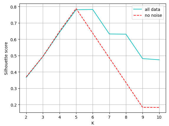
Note how the presence of outliers affects the Silhouette: although the clusterings produced have an excessive value of K (we know that N = 5 should be ideal), the Silhouette drops quite slowly. Why does that happen?

We hope that this has been a useful post for you to (i) get an idea about what a selection test for MALTO looks like and (ii) learn something new about computer science, statistics and ML-related topics!

Flavio Giobergia

Share on

Twitter Facebook LinkedIn